pacman::p_load(tmap, tidyverse, sf)Hands-on_Ex08B
Analytical Mapping
This document is about ploting analytical maps with the following steps:
Importing geospatial data in rds format into R environment.
Creating cartographic quality choropleth maps by using appropriate tmap functions.
Creating rate map
Creating percentile map
Creating boxmap
Load Library and Data
NGA_wp <- read_rds("data/rds/NGA_wp.rds")Basic Choropleth Mapping
  p1 <- tm_shape(NGA_wp) +
  tm_fill("wp_functional",
          n = 10,
          style = "equal",
          palette = "Blues") +
  tm_borders(lwd = 0.1,
             alpha = 1) +
  tm_layout(main.title = "Distribution of functional water point by LGAs",
            legend.outside = FALSE)

  p2 <- tm_shape(NGA_wp) +
  tm_fill("total_wp",
          n = 10,
          style = "equal",
          palette = "Blues") +
  tm_borders(lwd = 0.1,
             alpha = 1) +
  tm_layout(main.title = "Distribution of total  water point by LGAs",
            legend.outside = FALSE)

  tmap_arrange(p2, p1, nrow = 1)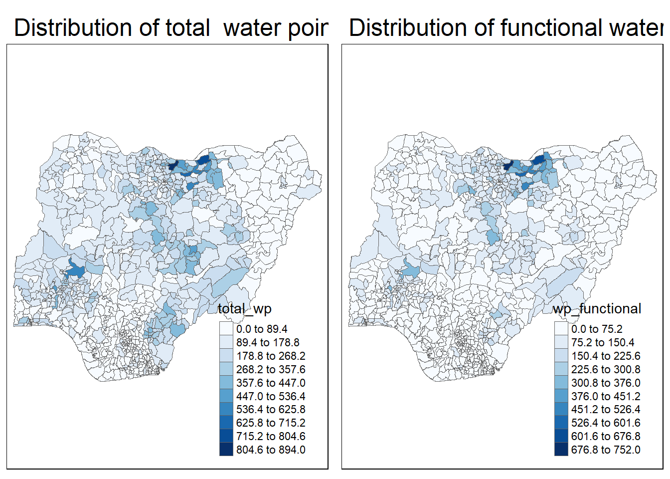
Deriving Proportion of Functional Water Points and Non-Functional Water Points
We will tabulate the proportion of functional water points and the proportion of non-functional water points in each LGA. In the following code chunk, mutate() from dplyr package is used to derive two fields, namely pct_functional and pct_nonfunctional.
  NGA_wp <- NGA_wp %>%
    mutate(pct_functional = wp_functional/total_wp) %>%
    mutate(pct_nonfunctional = wp_nonfunctional/total_wp)
map of rate
tm_shape(NGA_wp) +
  tm_fill("pct_functional",
          n = 10,
          style = "equal",
          palette = "Blues",
          legend.hist = TRUE) +
  tm_borders(lwd = 0.1,
             alpha = 1) +
  tm_layout(main.title = "Rate map of functional water point by LGAs",
            legend.outside = TRUE)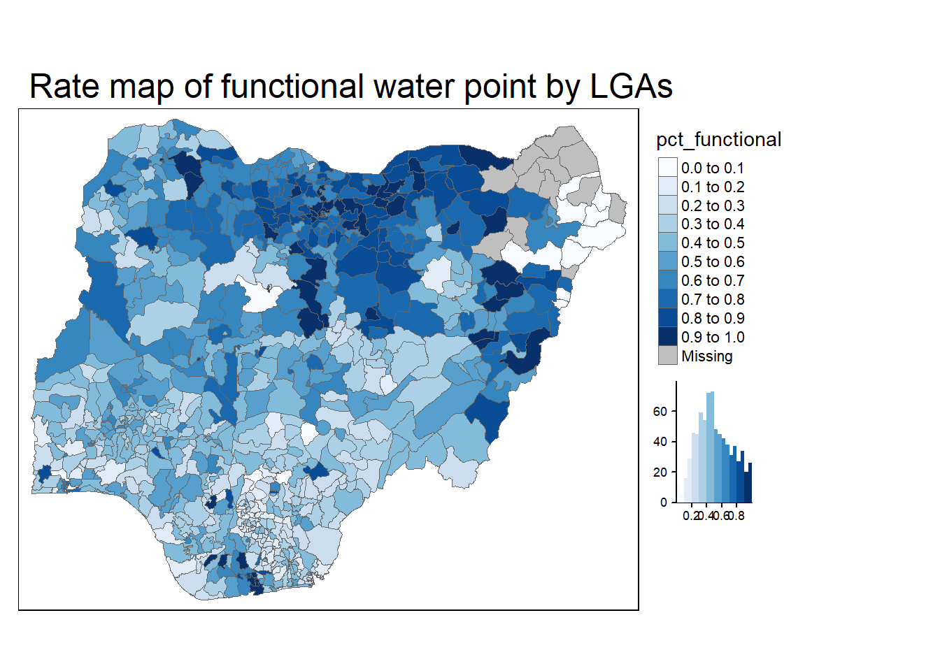
Percentile Map
The percentile map is a special type of quantile map with six specific categories: 0-1%,1-10%, 10-50%,50-90%,90-99%, and 99-100%. The corresponding breakpoints can be derived by means of the base R quantile command, passing an explicit vector of cumulative probabilities as c(0,.01,.1,.5,.9,.99,1). Note that the begin and endpoint need to be included.
It’s important to have 0 and 1 at the two ends.
We need to drop the drometry
Data Preparation
Step 1: Exclude records with NA by using the code chunk below.
NGA_wp <- NGA_wp %>% drop_na()Step 2: Creating customised classification and extracting values
  percent <- c(0,.01,.1,.5,.9,.99,1)
  var <- NGA_wp["pct_functional"] %>%
  st_set_geometry(NULL) #this is to drop away the column geometry
quantile(var[,1], percent)
0% 1% 10% 50% 90% 99% 100%
0.0000000 0.0000000 0.2169811 0.4791667 0.8611111 1.0000000 1.0000000 Creating the get.var function
Firstly, we will write an R function as shown below to extract a variable (i.e. wp_nonfunctional) as a vector out of an sf data.frame.
- arguments:
- vname: variable name (as character, in quotes)
- df: name of sf data frame
- returns:
- v: vector with values (without a column name)
  get.var <- function(vname,df) {
    v <- df[vname] %>%
    st_set_geometry(NULL)  #this is similar to drop the geometry column
  v <- unname(v[,1])
  return(v)
  }
A percentile mapping function
Next, we will write a percentile mapping function by using the code chunk below.
  #here we write another funciton and later we will reuse it
  percentmap <- function(vnam, df, legtitle=NA, mtitle="Percentile Map"){
  percent <- c(0,.01,.1,.5,.9,.99,1) #define percent cutting
  var <- get.var(vnam, df) #run the funtion to create variable
  bperc <- quantile(var, percent) #this is the quantile created
  tm_shape(df) +
  tm_polygons() +
  tm_shape(df) +
     tm_fill(vnam, #input parameter
             title=legtitle,
             breaks=bperc, #the pair we created using function earlier
             palette="Blues",
          labels=c("< 1%", "1% - 10%", "10% - 50%", "50% - 90%", "90% - 99%", "> 99%"))  +
  tm_borders() +
  tm_layout(main.title = mtitle,
            title.position = c("right","bottom"))
} percentmap("total_wp", NGA_wp)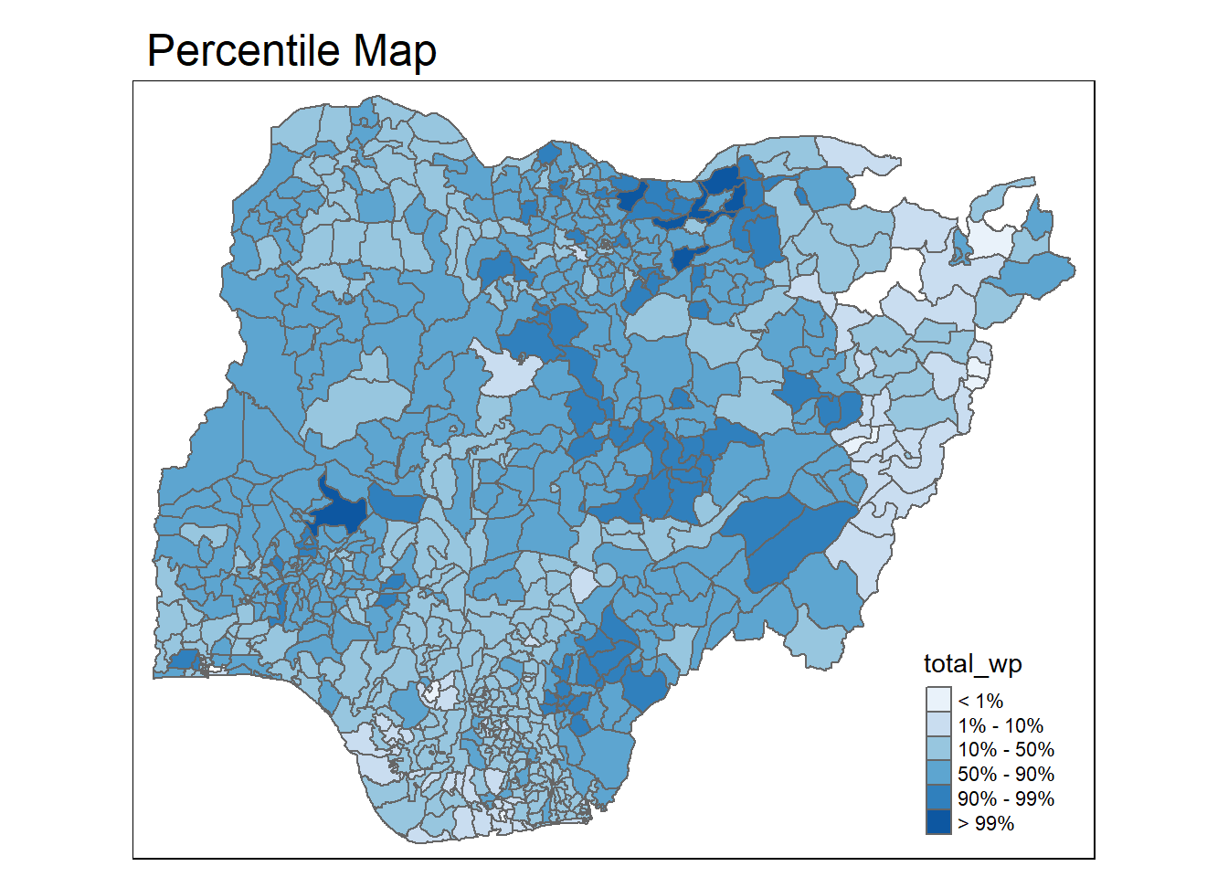
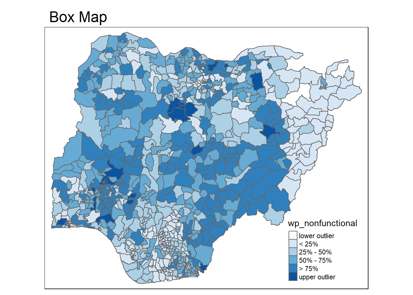
Box map
First, this is hoow it looks like when we plot normal boxplot:
  ggplot(data = NGA_wp,
       aes(x = "",
           y = wp_nonfunctional)) +
  geom_boxplot()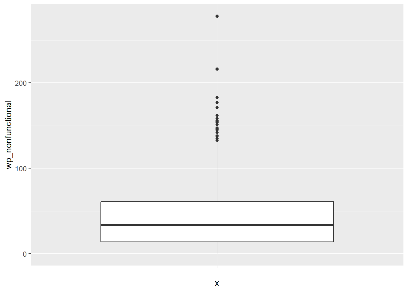
Creating the boxbreaks function
The code chunk below is an R function that creating break points for a box map.
arguments:
v: vector with observations
mult: multiplier for IQR (default 1.5)
returns:
- bb: vector with 7 break points compute quartile and fences
  boxbreaks <- function(v,mult=1.5) {
  qv <- unname(quantile(v)) #get the quatile value
  iqr <- qv[4] - qv[2] #calclating inter quantile range
  upfence <- qv[4] + mult * iqr
  lofence <- qv[2] - mult * iqr
  # initialize break points vector
  bb <- vector(mode="numeric",length=7)
  # logic for lower and upper fences
  if (lofence < qv[1]) {  # no lower outliers
    bb[1] <- lofence
    bb[2] <- floor(qv[1])
  } else {
    bb[2] <- lofence
    bb[1] <- qv[1]
  }
  if (upfence > qv[5]) { # no upper outliers
    bb[7] <- upfence
    bb[6] <- ceiling(qv[5])
  } else {
    bb[6] <- upfence
    bb[7] <- qv[5]
  }
  bb[3:5] <- qv[2:4]
  return(bb)
  }
Creating the get.var function
The code chunk below is an R function to extract a variable as a vector out of an sf data frame.
arguments:
vname: variable name (as character, in quotes)
df: name of sf data frame
returns:
- v: vector with values (without a column name)
  get.var <- function(vname,df) {
  v <- df[vname] %>% st_set_geometry(NULL)
  v <- unname(v[,1])
  return(v)
  }
Test and use the function
  var <- get.var("wp_nonfunctional", NGA_wp)
  boxbreaks(var)
[1] -56.5 0.0 14.0 34.0 61.0 131.5 278.0Boxmap function
The code chunk below is an R function to create a box map. - arguments: - vnam: variable name (as character, in quotes) - df: simple features polygon layer - legtitle: legend title - mtitle: map title - mult: multiplier for IQR - returns: - a tmap-element (plots a map)
  boxmap <- function(vnam, df,
                   legtitle=NA,
                   mtitle="Box Map",
                   mult=1.5){
  var <- get.var(vnam,df)
  bb <- boxbreaks(var)
  tm_shape(df) +
    tm_polygons() +
  tm_shape(df) +
     tm_fill(vnam,title=legtitle,
             breaks=bb,
             palette="Blues",
          labels = c("lower outlier",
                     "< 25%",
                     "25% - 50%",
                     "50% - 75%",
                     "> 75%",
                     "upper outlier"))  +
  tm_borders() +
  tm_layout(main.title = mtitle,
            title.position = c("left",
                               "top"))
} tmap_mode("plot")tmap mode set to plotting boxmap("wp_nonfunctional", NGA_wp)Warning: Breaks contains positive and negative values. Better is to use
diverging scale instead, or set auto.palette.mapping to FALSE.